1 – Quick EDA
The UCI Mushroom dataset consists of the following predictors and the liberty has been taken to name them as such in the assessment’s associated R-code.
Table 1 - UCI Mushroom Dataset Predictors
| No | Predictor Name and possible values | Type |
|---|---|---|
| 1 | cap-shape: bell=b,conical=c,convex=x,flat=f, knobbed=k,sunken=s | Categorical |
| 2 | cap-surface: fibrous=f,grooves=g,scaly=y,smooth=s | Categorical |
| 3 | cap-color: brown=n,buff=b,cinnamon=c,gray=g,green=r, pink=p,purple=u,red=e,white=w,yellow=y | Categorical |
| 4 | bruises: bruises=t,no=f | Categorical |
| 5 | odor: almond=a,anise=l,creosote=c,fishy=y,foul=f, musty=m,none=n,pungent=p,spicy=s | Categorical |
| 6 | gill-attachment: attached=a,descending=d,free=f,notched=n | Categorical |
| 7 | gill-spacing: close=c,crowded=w,distant=d | Categorical |
| 8 | gill-size: broad=b,narrow=n | Categorical |
| 9 | gill-color: black=k,brown=n,buff=b,chocolate=h,gray=g, green=r,orange=o,pink=p,purple=u,red=e, white=w,yellow=y | Categorical |
| 10 | stalk-shape: enlarging=e,tapering=t | Categorical |
| 11 | stalk-root: bulbous=b,club=c,cup=u,equal=e, rhizomorphs=z,rooted=r,missing=? | Categorical |
| 12 | stalk-surface-above-ring: fibrous=f,scaly=y,silky=k,smooth=s | Categorical |
| 13 | stalk-surface-below-ring: fibrous=f,scaly=y,silky=k,smooth=s | Categorical |
| 14 | stalk-color-above-ring: brown=n,buff=b,cinnamon=c,gray=g,orange=o, pink=p,red=e,white=w,yellow=y | Categorical |
| 15 | stalk-color-below-ring: brown=n,buff=b,cinnamon=c,gray=g,orange=o, pink=p,red=e,white=w,yellow=y | Categorical |
| 16 | veil-type: partial=p,universal=u | Categorical |
| 17 | veil-color: brown=n,orange=o,white=w,yellow=y | Categorical |
| 18 | ring-number: none=n,one=o,two=t | Categorical |
| 19 | ring-type: cobwebby=c,evanescent=e,flaring=f,large=l, none=n,pendant=p,sheathing=s,zone=z | Categorical |
| 20 | spore-print-color: black=k,brown=n,buff=b,chocolate=h,green=r, orange=o,purple=u,white=w,yellow=y | Categorical |
| 21 | population: abundant=a,clustered=c,numerous=n, scattered=s,several=v,solitary=y | Categorical |
| 22 | habitat: grasses=g,leaves=l,meadows=m,paths=p, urban=u,waste=w,woods=d | Categorical |
The UCI Mushroom dataset contains one dependant variable as listed in Table 2:
Table 2 - UCI Mushroom Dataset - Dependant Varible
| No | Dependant variable and possible values | Type |
|---|---|---|
| 1 | class: e=edible, p=poisonous | Categorical |
The UCI Mushroom dataset contains 8124 observations.
2 - Implementation Methodology for Wrapper Naïve Bayes
The naive_bayes() function in the naivebayes package was used to implement the wrapper. The dataset was read in directly from the UCI website and column names as listed in Table 1 and Table 2 were assigned upon consuming the data.
The wrapper was implemented according to a forward stepwise subset selection (prune later scheme). A utility function called, calc_classifier_error (see APPENDIX B), was implemented, that randomly split each candidate classifier’s data into a training subset and a test subset containing 80% and 20% of the observations, respectively. This procedure was repeated 10 times – each time calculating the prediction error for the classifier - the final error of the candidate classifier was then averaged over the 10 attempts and used to rank the classifier against other candidate classifiers.
An initial run was performed to calculate what the average classification errors were for when each predictor was used on its own. For example:
class ~ cap-shape,
class ~ cap-surface,
class ~ cap_color,
etc.
The error list obtained from this step was ordered in ascending order. This list served as input to a second process, which iteratively built formula strings that served as subsets of features from which classifier were generated. From this list the predictor with the smallest error (top of the list) was placed in the first position of the formula string and then each subsequent predictor was in turn added to the string and then applied to the naïve_bayes() function. For example:
class ~ odor + cap-shape,
class ~ odor + cap-surface,
class ~ odor + cap-color,
etc.
All the errors that were calculated for these combinations were again captured in a list and ordered in ascending order. The top candidate was then used as the initial base for the third iterations. For example:
class ~ odor + spore_print_color + stalk_color_above_ring,
class ~ odor + spore_print_color + ring_type,
etc.
This process was repeated iteratively until all the predictors were exhausted and a final ordered list was obtained. The full list can be viewed in APPENDIX – A. Plots were then generated for the ordered feature set |S| = 1, …, n. Refer to APPENDIX - B for the full R-code listing.
Essentially, two data frames of predictors are maintained during the forward iteration process. Top listed feature candidates are transferred from the one data frame to the other as they are tested. Candidate subsets are built for the next iteration by reading the features in a sequential order from the one list and then iteratively adding a next feature from the other list. The stop criteria are when the second list is exhausted, and the first list contains all of the features and ranked in order. This means the first feature in the data frame would be considered the most efficient feature when measured on its own (|S|=1). The second feature would be considered the most effective when measured in conjunction with the first feature (|S| = 1+2). The third feature would be considered the most effective when measured in conjunction with the first and second features (|S|=1+2+3), etc.
3 – Results
Figure 1 displays the average classification error for each predictor tested individually. The predictor number on the x-axis corresponds to the numbers in Table 1. From Figure 1 it can be clearly observed that predictor no.5 (odor, as listed in Table 1), is the feature that resulted in the smallest classification error – 0.15%. This feature alone fares much better compared to the whole feature set of 22 features that yielded a classification error of 0.4%. The top three features from Figure 1 are:
-
5 – Odor – 0.15%
-
20 – Spore Print Color – 1.34%
-
9 – Gill Color – 1.84%
The rest of the features all produce individual classification error rates of between 2% and 5%.
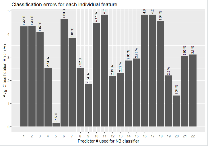
Figure 1 - Individual predictor errors
Plotting the fully ordered feature set as obtained from the output in APPENDIX – A yields the following figure:
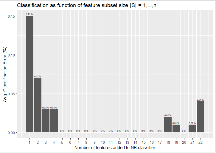
Figure 2 - Classification as function of feature subset |S|
From Figure 2 it can be observed what the overall classification error is for each addition of optimally selected feature that was sequentially added and tested. For example, the top feature that yielded the smallest classification error of 0.15% (feature no.5 - odor), is indicated by the bar positioned at 1 (subset 1: class ~ odor). The second bar indicates the second subset’s cumulative classification error (subset 2: class ~ odor + spore_print_color), which reduces the classification error to 0.07%. By adding a third predictor, the classification error is again reduced by half to yield an error of only 0.03%. From this we can draw the conclusion that by optimally selecting features a classification error of at least an order of magnitude better can be achieved by a mere 3 features (subset 3: class ~ odor + spore_print_color + stalk_color_above_ring) against a full feature set of 22. From a statistical point of view one can safely deduce that these three features are the most statistically relevant features in the set of 22 features.
As additional features are added to the subsets it can be observed that between the 5th and 17th feature added, the classifiers reach a 0% average error rate. Might this be due to overfitting? From the 18th to the 22nd feature added to the model one can see that non-zero error rates are starting to occur again. This could indicate that the model has become too complex again and therefore less efficient.
The output in APPENDIX-A suggests that the most optimal feature selection candidate is subset 5, which yields a classification error of 0% by utilising only the following five features (Subset (S)):
class ~ odor + spore_print_color + stalk_color_above_ring + ring_type + stalk_surface_above_ring
The above subset of features is easier to understand and grasp and makes it a lot easier to identify edible mushrooms when one is roaming around in the great outdoors. In fact, if one had to choose only one feature then it would be odor (predictor no.5). Like the saying goes, “If it smells off, then don’t eat it…” That way I have 0.15% chance of incorrectly identifying a poisonous mushroom. And, in the words of one of the greatest philosophers of all time – Homer Simpson, “I like those odds.”
Alternative to the brut-force method applied via the forward stepwise subset selection - prune later scheme, one can contemplate applying statistical tests of significance to the set of 22 features. One such scheme, for instance, might very well be χ2-test. The χ2-test, according to popular demand, is highly suitable for determining statistical significance on features sets that are of the categorical type.
The conclusion regarding this experiment is that more = less. Only a small subset of the features (<30%) has proven to be statistically significant enough to produce a near zero classification error rate.
Bonus: As an additional thought, it would be interesting to see if cluster analysis would be able to identify clusters of mushrooms with similar traits? If so, what would those cluster signify? Different mushroom species?
APPENDIX – A
[1] “Iteration: 2”
[1] “Subset(S): class ~ odor + spore_print_color”
[1] “Avg. Error: 0.00073891625615764 ( 0.07 %)”
[1] “———————————-“
[1] “Iteration: 3”
[1] “Subset(S): class ~ odor + spore_print_color + stalk_color_above_ring”
[1] “Avg. Error: 0.00030788177339901 ( 0.03 %)”
[1] “———————————-“
[1] “Iteration: 4”
[1] “Subset(S): class ~ odor + spore_print_color + stalk_color_above_ring + ring_type”
[1] “Avg. Error: 0.00030788177339901 ( 0.03 %)”
[1] “———————————-“
[1] “Iteration: 5”
[1] “Subset(S): class ~ odor + spore_print_color + stalk_color_above_ring + ring_type + stalk_surface_above_ring”
[1] “Avg. Error: 0 ( 0 %)”
[1] “———————————-“
[1] “Iteration: 6”
[1] “Subset(S): class ~ odor + spore_print_color + stalk_color_above_ring + ring_type + stalk_surface_above_ring + veil_color”
[1] “Avg. Error: 0 ( 0 %)”
[1] “———————————-“
[1] “Iteration: 7”
[1] “Subset(S): class ~ odor + spore_print_color + stalk_color_above_ring + ring_type + stalk_surface_above_ring + veil_color + ring_number”
[1] “Avg. Error: 0 ( 0 %)”
[1] “———————————-“
[1] “Iteration: 8”
[1] “Subset(S): class ~ odor + spore_print_color + stalk_color_above_ring + ring_type + stalk_surface_above_ring + veil_color + ring_number + veil_type”
[1] “Avg. Error: 0 ( 0 %)”
[1] “———————————-“
[1] “Iteration: 9”
[1] “Subset(S): class ~ odor + spore_print_color + stalk_color_above_ring + ring_type + stalk_surface_above_ring + veil_color + ring_number + veil_type + bruises”
[1] “Avg. Error: 0 ( 0 %)”
[1] “———————————-“
[1] “Iteration: 10”
[1] “Subset(S): class ~ odor + spore_print_color + stalk_color_above_ring + ring_type + stalk_surface_above_ring + veil_color + ring_number + veil_type + bruises + cap_surface”
[1] “Avg. Error: 0 ( 0 %)”
[1] “———————————-“
[1] “Iteration: 11”
[1] “Subset(S): class ~ odor + spore_print_color + stalk_color_above_ring + ring_type + stalk_surface_above_ring + veil_color + ring_number + veil_type + bruises + cap_surface + cap_color”
[1] “Avg. Error: 0 ( 0 %)”
[1] “———————————-“
[1] “Iteration: 12”
[1] “Subset(S): class ~ odor + spore_print_color + stalk_color_above_ring + ring_type + stalk_surface_above_ring + veil_color + ring_number + veil_type + bruises + cap_surface + cap_color + stalk_root”
[1] “Avg. Error: 0 ( 0 %)”
[1] “———————————-“
[1] “Iteration: 13”
[1] “Subset(S): class ~ odor + spore_print_color + stalk_color_above_ring + ring_type + stalk_surface_above_ring + veil_color + ring_number + veil_type + bruises + cap_surface + cap_color + stalk_root + population”
[1] “Avg. Error: 0 ( 0 %)”
[1] “———————————-“
[1] “Iteration: 14”
[1] “Subset(S): class ~ odor + spore_print_color + stalk_color_above_ring + ring_type + stalk_surface_above_ring + veil_color + ring_number + veil_type + bruises + cap_surface + cap_color + stalk_root + population + gill_attachment”
[1] “Avg. Error: 0 ( 0 %)”
[1] “———————————-“
[1] “Iteration: 15”
[1] “Subset(S): class ~ odor + spore_print_color + stalk_color_above_ring + ring_type + stalk_surface_above_ring + veil_color + ring_number + veil_type + bruises + cap_surface + cap_color + stalk_root + population + gill_attachment + gill_color”
[1] “Avg. Error: 0 ( 0 %)”
[1] “———————————-“
[1] “Iteration: 16”
[1] “Subset(S): class ~ odor + spore_print_color + stalk_color_above_ring + ring_type + stalk_surface_above_ring + veil_color + ring_number + veil_type + bruises + cap_surface + cap_color + stalk_root + population + gill_attachment + gill_color + stalk_shape”
[1] “Avg. Error: 0 ( 0 %)”
[1] “———————————-“
[1] “Iteration: 17”
[1] “Subset(S): class ~ odor + spore_print_color + stalk_color_above_ring + ring_type + stalk_surface_above_ring + veil_color + ring_number + veil_type + bruises + cap_surface + cap_color + stalk_root + population + gill_attachment + gill_color + stalk_shape + habitat”
[1] “Avg. Error: 0 ( 0 %)”
[1] “———————————-“
[1] “Iteration: 18”
[1] “Subset(S): class ~ odor + spore_print_color + stalk_color_above_ring + ring_type + stalk_surface_above_ring + veil_color + ring_number + veil_type + bruises + cap_surface + cap_color + stalk_root + population + gill_attachment + gill_color + stalk_shape + habitat + stalk_surface_below_ring”
[1] “Avg. Error: 0.000184729064039413 ( 0.02 %)”
[1] “———————————-“
[1] “Iteration: 19”
[1] “Subset(S): class ~ odor + spore_print_color + stalk_color_above_ring + ring_type + stalk_surface_above_ring + veil_color + ring_number + veil_type + bruises + cap_surface + cap_color + stalk_root + population + gill_attachment + gill_color + stalk_shape + habitat + stalk_surface_below_ring + gill_spacing”
[1] “Avg. Error: 0.000123152709359609 ( 0.01 %)”
[1] “———————————-“
[1] “Iteration: 20”
[1] “Subset(S): class ~ odor + spore_print_color + stalk_color_above_ring + ring_type + stalk_surface_above_ring + veil_color + ring_number + veil_type + bruises + cap_surface + cap_color + stalk_root + population + gill_attachment + gill_color + stalk_shape + habitat + stalk_surface_below_ring + gill_spacing + gill_size”
[1] “Avg. Error: 0 ( 0 %)”
[1] “———————————-“
[1] “Iteration: 21”
[1] “Subset(S): class ~ odor + spore_print_color + stalk_color_above_ring + ring_type + stalk_surface_above_ring + veil_color + ring_number + veil_type + bruises + cap_surface + cap_color + stalk_root + population + gill_attachment + gill_color + stalk_shape + habitat + stalk_surface_below_ring + gill_spacing + gill_size + cap_shape”
[1] “Avg. Error: 0.000123152709359609 ( 0.01 %)”
[1] “———————————-“
[1] “Iteration: 22”
[1] “Subset(S): class ~ odor + spore_print_color + stalk_color_above_ring + ring_type + stalk_surface_above_ring + veil_color + ring_number + veil_type + bruises + cap_surface + cap_color + stalk_root + population + gill_attachment + gill_color + stalk_shape + habitat + stalk_surface_below_ring + gill_spacing + gill_size + cap_shape + stalk_color_below_ring”
[1] “Avg. Error: 0.000369458128078815 ( 0.04 %)”
[1] “———————————-“